Midterm Review
Sarah Jewett
library(stargazer)
library(dplyr)
library(ggplot2)
data("Auto", package = "ISLR")
Auto$name <- as.factor(Auto$name)
Regression
Predicted Probabilities
Say we want to see the predicted probabilities for the first few rows of the Auto data based on a linear regression model with only two independent variables:
lm.1 <- lm(mpg ~ cylinders + weight, Auto)
summary(lm.1)
##
## Call:
## lm(formula = mpg ~ cylinders + weight, data = Auto)
##
## Residuals:
##      Min       1Q   Median       3Q      Max
## -12.6469  -2.8282  -0.2905   2.1606  16.5856
##
## Coefficients:
##               Estimate Std. Error t value Pr(>|t|)
## (Intercept) 46.2923105  0.7939685  58.305   <2e-16 ***
## cylinders   -0.7213779  0.2893780  -2.493   0.0131 *
## weight      -0.0063471  0.0005811 -10.922   <2e-16 ***
## ---
## Signif. codes:  0 '***' 0.001 '**' 0.01 '*' 0.05 '.' 0.1 ' ' 1
##
## Residual standard error: 4.304 on 389 degrees of freedom
## Multiple R-squared:  0.6975, Adjusted R-squared:  0.6959
## F-statistic: 448.4 on 2 and 389 DF,  p-value: < 2.2e-16
We can use predict() to see what the car’s predicted mpg is based on the above coefficients
predict(lm.1, newdata = Auto[1:6,], type = "response")
##        1        2        3        4        5        6
## 18.28101 17.08141 18.71261 18.73166 18.63010 12.96848
# OR
lm.1$fitted.values[1:6]
##        1        2        3        4        5        6
## 18.28101 17.08141 18.71261 18.73166 18.63010 12.96848
Our predicted MPG for the first row is 18.28101
Let’s see how we get this predicted MPG:
First we pull out the relevant coefficients from lm.1:
intercept      <- 46.2923105
beta_cylinders <- -0.7213779
beta_weight    <- -0.0063471

# OR

intercept      <- lm.1$coefficients[1]
beta_cylinders <- lm.1$coefficients[2]
beta_weight    <- lm.1$coefficients[3]
This is: MPG = 46.29 + -0.72*cylinders + –0.006*weight
Let’s take a look at the first row and see what the values are in the data:
Auto[1,]
##   mpg cylinders displacement horsepower weight acceleration year origin
## 1  18         8          307        130   3504           12   70      1
##                        name
## 1 chevrolet chevelle malibu
MPG = 46.29 + -0.7213779*8 + -0.0063471*3504
Our predicted MPG was: 18.28101 Does this match?
predicted_mpg <- intercept + beta_cylinders*Auto$cylinders[1] + beta_weight*Auto$weight[1]

unname(predicted_mpg)
## [1] 18.28101
# unname() takes away the name from 'Named number' values, which this is.
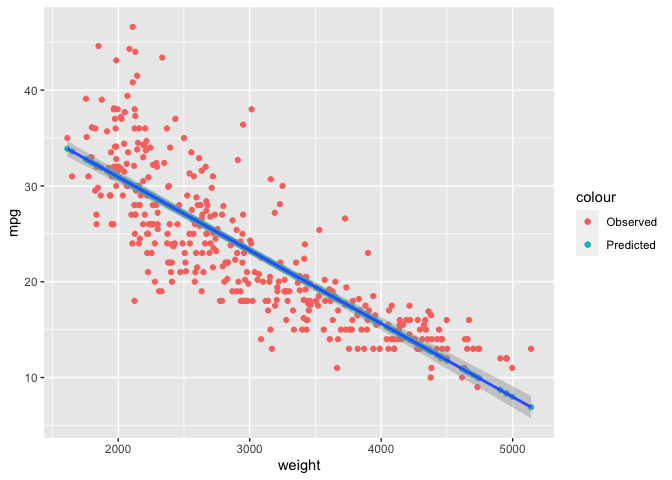
Now, we can have fun and easily plot our original mpg values with the fitted values. We will also add the regression line like in Assignment 3 to see how the predicted values plot compared to when we do lm() within a plot with our data.
lm.3 <- lm(mpg ~ weight, Auto)
summary(lm.3)
##
## Call:
## lm(formula = mpg ~ weight, data = Auto)
##
## Residuals:
##      Min       1Q   Median       3Q      Max
## -11.9736  -2.7556  -0.3358   2.1379  16.5194
##
## Coefficients:
##              Estimate Std. Error t value Pr(>|t|)
## (Intercept) 46.216524   0.798673   57.87   <2e-16 ***
## weight      -0.007647   0.000258  -29.64   <2e-16 ***
## ---
## Signif. codes:  0 '***' 0.001 '**' 0.01 '*' 0.05 '.' 0.1 ' ' 1
##
## Residual standard error: 4.333 on 390 degrees of freedom
## Multiple R-squared:  0.6926, Adjusted R-squared:  0.6918
## F-statistic: 878.8 on 1 and 390 DF,  p-value: < 2.2e-16
Auto$pred <- unname(lm.3$fitted.values)

ggplot(Auto, aes(y = mpg, x = weight)) +
  geom_point(aes(color = "Observed")) +
  geom_point(aes(y = pred, color = "Predicted")) +
  geom_smooth(method = lm)
## `geom_smooth()` using formula = 'y ~ x'
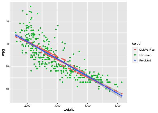
Now if we want to start looking at how adding variables changes from the original regression line we can add points from our earlier regression on mpg with weight and cylinders
Auto$pred2 <- unname(lm.1$fitted.values)

ggplot(Auto, aes(y = mpg, x = weight)) +
  geom_point(aes(color = "Observed")) +
  geom_point(aes(y = pred, color = "Predicted")) +
  geom_point(aes(y=pred2, color = "MultiVarReg")) +
    geom_smooth(method = lm)
## `geom_smooth()` using formula = 'y ~ x'
Interactions!
When don’t use interactions, we are assuming that the independent variables are, well, independent to each other. An interaction is looking at, say, how x1’s impact on y depends on x1’s relationship with x2.
Imagine we are looking at whether people like peanut butter or jelly. If we only look at the two spreads independently, we might miss that many people actual PREFER to eat peanut butter and jelly together and that their level of enjoyment increases when they eat them together.
If we have a sample from a survey of people across a few days days at a hotel asking if they enjoyed their breakfast or not, we can see how this PB&J situation might look in the data. Imagine we also asked what they ate for breakfast, with a bunch of foods including peanut butter and jelly. We also know that on one day that they ran out of peanut butter at some point and on another day, they ran out of jelly.
Enjoyment is measured from 1-10, with 6 being the threshold for being able to say they enjoyed the meal. (This is just to avoid a binary dependent variable, even though we are going to more or less consider it as such).
So say we have: 12 people who ate PB & Jelly (all but 1 enjoyed their breakfast) 5 people who ate PB (1 enjoyed their breakfast) 5 people who ate jelly (4 enjoyed their breakfast) 4 people who ate neither (and all enjoyed their breakfast)
We create a data frame:
food <- data.frame(PB =    c(1, 1, 1, 1, 1, 1, 1, 1, 1, 1, 1, 1,  1, 1, 1, 1, 1,  0, 0, 0, 0, 0,  0, 0, 0, 0),
                   Jelly = c(1, 1, 1, 1, 1, 1, 1, 1, 1, 1, 1, 1,  0, 0, 0, 0, 0,  1, 1, 1, 1, 1,  0, 0, 0, 0),
                   Enjoy = c(8, 7, 9, 3, 8, 9, 9, 6, 8, 6, 7, 8,  1, 5, 6, 2, 3,  7, 7, 3, 9, 8,  7, 8, 6, 8))
And now we can run three different linear models, two of which include interactions.
- Using * will run a model with independent variables AND the interaction
- Using : will remove the independent variables from the model and only look at the interaction
So if we decide to look at the impact of whether a person had peanut butter and jelly on their enjoyment rating…
First a basic regression
lm.no_inter <- lm(Enjoy ~ Jelly + PB, food)
This keeps the independent variables and the interactions (identical ways of doing this but with * and :)
lm.all_inter <-   lm(Enjoy ~ Jelly * PB, food)
lm.all_inter2 <-  lm(Enjoy ~ Jelly + PB + Jelly:PB, food)
but not the same as:
lm.inter_only <- lm(Enjoy ~ Jelly:PB, food)
Let’s look at them side by side (using stargazer package, shows in knit HTML only):
stargazer(lm.no_inter, lm.all_inter, lm.inter_only, type = "html")
| Dependent variable: | |||
| Enjoy | |||
| \(1\) | \(2\) | \(3\) | |
| Jelly | 2.240\*\* | -0.450 | |
| (0.868) | (1.225) | ||
| PB | -1.160 | -3.850\*\*\* | |
| (0.868) | (1.225) | ||
| Jelly:PB | 4.383\*\* | 1.619\* | |
| (1.564) | (0.863) | ||
| Constant | 5.756\*\*\* | 7.250\*\*\* | 5.714\*\*\* |
| (0.845) | (0.913) | (0.586) | |
| Observations | 26 | 26 | 26 |
| R2 | 0.248 | 0.446 | 0.128 |
| Adjusted R2 | 0.183 | 0.370 | 0.092 |
| Residual Std. Error | 2.081 (df = 23) | 1.827 (df = 22) | 2.194 (df = 24) |
| F Statistic | 3.792\*\* (df = 2; 23) | 5.898\*\*\* (df = 3; 22) | 3.519\* (df = 1; 24) |
| Note: | *p\<0.1; **p\<0.05; ***p\<0.01 | ||
So the regression output, without the interaction, shows a negative relationship with PB and enjoyment. However, we know in the observed data, that people who had peanut butter AND jelly, enjoyed their breakfast except for one person. This can lead us to believe that having PB on it’s own will lead to lower ratings of breakfast enjoyment, which isn’t untrue if you look only at the people who ate just peanut butter. In short, this isn’t capturing the relationship between PB & Jelly as a combination in enjoyment.
When we look at the regression with the interaction, we can see that suddenly the relationship with enjoyment and PB becomes worse, BUT the interaction rightfully captures that many people who had PB & J enjoyed their meal more. So in this sense, it is illustrating that when people have PB on its own, they they tend to enjoy their meal less, but when they have PB & J together, they are more likely to enjoy their meal.
You can look at jelly the same way – without the interaction, having jelly has a positive relationship with enjoyment. But with the interaction, it actually gets worse, even though for the most part, people enjoyed their meal when only having jelly.
We can further demystify this by looking at the predicted probability of a specific case, in this instance, the first row observation in the data we created which is someone who had peanut butter and jelly.
predicted.ind <- lm.no_inter$coefficients[1] + # this is the constant/intercept
                 lm.no_inter$coefficients[2]*food$Jelly[1] + # this is beta of Jelly * Jelly (observed)
                 lm.no_inter$coefficients[3]*food$PB[1] # this is beta of PB * PB (observed)

predicted.ind_int <- lm.all_inter$coefficients[1] + # this is the constant/intercept
                     lm.all_inter$coefficients[2]*food$Jelly[1] + #  # this is beta of Jelly * Jelly (observed)
                     lm.all_inter$coefficients[3]*food$PB[1] + # this is beta of PB * PB (observed)
                     lm.all_inter$coefficients[4]*food$Jelly[1]*food$PB[1] # this is beta of interaction * Jelly (observed) AND * PB (observed)

sprintf("The non-interaction model shows a predicted rating of %g for PB&J and the model with the interaction shows a predicted rating of %g for PB&J\n",
        unname(predicted.ind), unname(predicted.ind_int)) %>%
    cat()
## The non-interaction model shows a predicted rating of 6.83523 for PB&J and the model with the interaction shows a predicted rating of 7.33333 for PB&J
So what about if they only had jelly, what is the predicted enjoyment rating?
Easier to just create a new df with the 4 possibilities and see the predictions using pred()
new_food <- data.frame(PB    = c(1, 1, 0, 0),
                       Jelly = c(1, 0, 1, 0))

predict(lm.no_inter, new_food, type = "response")
##        1        2        3        4
## 6.835227 4.595455 7.995455 5.755682
# Highest predicted rating goes to Jelly only here
predict(lm.all_inter, new_food, type = "response")
##        1        2        3        4
## 7.333333 3.400000 6.800000 7.250000
# Highest predicted rating goes to PB & J here
This is showing that without the interaction, people having only jelly are predicted to have a higher enjoyment rating on average than those who had both peanut butter and jelly.
The interaction model, however, adjusts for this relationship between the two. So the now negative coefficient for jelly actually brings the predicted rating down to 6.8, which is lower than the interaction model for PB & J (7.33)
This is a saturated model so you may have noticed that the predicted ratings for the interaction model match the mean for each of the four possible options. We can see what the observed means for the four groupings like so:
enjoy_mean <- food %>%
    group_by(across(c(PB, Jelly))) %>%
    summarize(Mean = mean(Enjoy))
## `summarise()` has grouped output by 'PB'. You can override using the `.groups`
## argument.
enjoy_mean
## # A tibble: 4 × 3
## # Groups:   PB [2]
##      PB Jelly  Mean
##   <dbl> <dbl> <dbl>
## 1     0     0  7.25
## 2     0     1  6.8
## 3     1     0  3.4
## 4     1     1  7.33
Manipulating your observations before regressing:
Say we wanted to take all of the numeric values and sqrt them before running the regression. There are a number of reasons why you might want to do this, which you can read about here.
A long way:
sqrt_Auto <- Auto %>%
  mutate(sqrt_mpg = sqrt(mpg)) %>%
  mutate(sqrt_cylinders = sqrt(cylinders)) %>%
  mutate(sqrt_displacement = sqrt(displacement)) %>%
  mutate(sqrt_horsepower = sqrt(horsepower)) %>%
  mutate(sqrt_weight = sqrt(weight)) %>%
  mutate(sqrt_acceleration = sqrt(acceleration))

head(sqrt_Auto)
##   mpg cylinders displacement horsepower weight acceleration year origin
## 1  18         8          307        130   3504         12.0   70      1
## 2  15         8          350        165   3693         11.5   70      1
## 3  18         8          318        150   3436         11.0   70      1
## 4  16         8          304        150   3433         12.0   70      1
## 5  17         8          302        140   3449         10.5   70      1
## 6  15         8          429        198   4341         10.0   70      1
##                        name     pred    pred2 sqrt_mpg sqrt_cylinders
## 1 chevrolet chevelle malibu 19.42024 18.28101 4.242641       2.828427
## 2         buick skylark 320 17.97489 17.08141 3.872983       2.828427
## 3        plymouth satellite 19.94026 18.71261 4.242641       2.828427
## 4             amc rebel sst 19.96320 18.73166 4.000000       2.828427
## 5               ford torino 19.84084 18.63010 4.123106       2.828427
## 6          ford galaxie 500 13.01941 12.96848 3.872983       2.828427
##   sqrt_displacement sqrt_horsepower sqrt_weight sqrt_acceleration
## 1          17.52142        11.40175    59.19459          3.464102
## 2          18.70829        12.84523    60.77006          3.391165
## 3          17.83255        12.24745    58.61740          3.316625
## 4          17.43560        12.24745    58.59181          3.464102
## 5          17.37815        11.83216    58.72819          3.240370
## 6          20.71232        14.07125    65.88627          3.162278
Or we can do it with dplyr’s across() function:
s_Auto <- Auto %>%
  mutate(across(c(mpg, cylinders, displacement, horsepower, weight, acceleration), sqrt, .names = "sqrt_{.col}"))

head(s_Auto)
##   mpg cylinders displacement horsepower weight acceleration year origin
## 1  18         8          307        130   3504         12.0   70      1
## 2  15         8          350        165   3693         11.5   70      1
## 3  18         8          318        150   3436         11.0   70      1
## 4  16         8          304        150   3433         12.0   70      1
## 5  17         8          302        140   3449         10.5   70      1
## 6  15         8          429        198   4341         10.0   70      1
##                        name     pred    pred2 sqrt_mpg sqrt_cylinders
## 1 chevrolet chevelle malibu 19.42024 18.28101 4.242641       2.828427
## 2         buick skylark 320 17.97489 17.08141 3.872983       2.828427
## 3        plymouth satellite 19.94026 18.71261 4.242641       2.828427
## 4             amc rebel sst 19.96320 18.73166 4.000000       2.828427
## 5               ford torino 19.84084 18.63010 4.123106       2.828427
## 6          ford galaxie 500 13.01941 12.96848 3.872983       2.828427
##   sqrt_displacement sqrt_horsepower sqrt_weight sqrt_acceleration
## 1          17.52142        11.40175    59.19459          3.464102
## 2          18.70829        12.84523    60.77006          3.391165
## 3          17.83255        12.24745    58.61740          3.316625
## 4          17.43560        12.24745    58.59181          3.464102
## 5          17.37815        11.83216    58.72819          3.240370
## 6          20.71232        14.07125    65.88627          3.162278
Note: Remove the ‘.names’ argument if you want to overwrite the columns